introduction

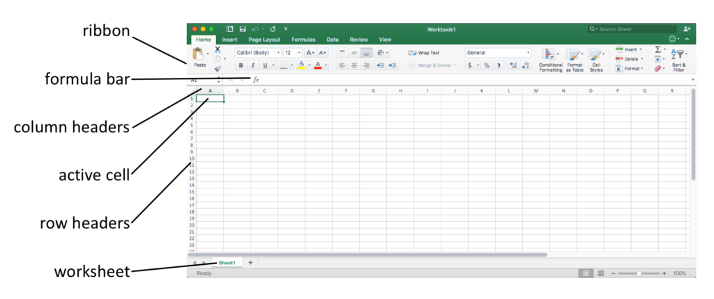
Microsoft Excel is a spreadsheet program that is used to record and analyse numerical data. Think of a spreadsheet as a collection of columns and rows that form a table. Alphabetical letters are usually assigned to columns and numbers are usually assigned to rows.

Use of excal

Excel is used to store, analyze, and report on large amounts of data. It is often used by accounting teams for financial analysis, but can be used by any professional to manage long and unwieldy datasets.

Funtion of excal

Function	Description
=AND	Returns TRUE or FALSE based on two or more conditions
=AVERAGE	Calculates the average (arithmetic mean)
=AVERAGEIF	Calculates the average of a range based on a TRUE or FALSE condition
=AVERAGEIFS	Calculates the average of a range based on one or more TRUE/FALSE conditions
=CONCAT	Links together the content of multiple cells
=COUNT	Counts cells with numbers in a range
=COUNTA	Counts all cells in a range that has values, both numbers and letters
=COUNTBLANK	Counts blank cells in a range
=COUNTIF	Counts cells as specified
=COUNTIFS	Counts cells in a range based on one or more TRUE or FALSE condition
=IF	Returns values based on a TRUE or FALSE condition
=IFS	Returns values based on one or more TRUE or FALSE conditions
=LEFT	Returns values from the left side of a cell
=LOWER	Reformats content to lowercase
=MAX	Returns the highest value in a range
=MEDIAN	Returns the middle value in the data
=MIN	Returns the lowest value in a range
=MODE	Finds the number seen most times. The function always returns a single number
=NPV	The NPV function is used to calculate the Net Present Value (NPV)
=OR	Returns TRUE or FALSE based on two or more conditions
=RAND	Generates a random number
=RIGHT	Returns values from the right side of a cell
=STDEV.P	Calculates the Standard Deviation (Std) for the entire population
=STDEV.S	Calculates the Standard Deviation (Std) for a sample
=SUM	Adds together numbers in a range
=SUMIF	Calculates the sum of values in a range based on a TRUE or FALSE condition
=SUMIFS	Calculates the sum of a range based on one or more TRUE or FALSE condition
=TRIM	Removes irregular spacing, leaving one space between each value
=VLOOKUP	Allows vertical searches for values in a table
=XOR	Returns TRUE or FALSE based on two or more conditions

what is data maintainance

Data maintenance is the process of auditing, organizing and correcting data in management systems and databases to ensure accuracy and accessibility. This process is important because it allows organizations to identify and correct issues before they become a more significant concern and enables them to prevent some problems from occurring. Data maintenance is a general term that encompasses many elements of data.

what is data clansing ?

Data cleansing, also known as data cleaning, is an element of data maintenance that involves identifying inaccurate data and fixing it to ensure the correct format and information. adjusting formatting to maintain consistency and removing special characters. You can perform data cleansing manually or by using specialized software.

what is use formula in excal

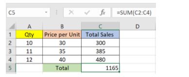
1.SUM

The SUM() function, as the name suggests, gives the total of the selected range of cell values. It performs the mathematical operation which is addition. Here’s an example of it below:

Sum “=SUM(C2:C4)”

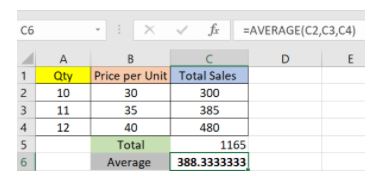
2.AVERAGE

The AVERAGE() function focuses on calculating the average of the selected range of cell values. As seen from the below example, to find the avg of the total sales, you have to simply type in:

AVERAGE =AVERAGE(C2, C3, C4)

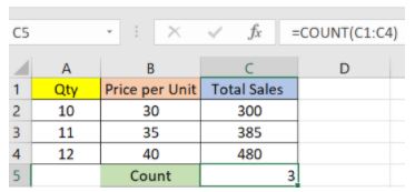
3.COUNT

The function COUNT() counts the total number of cells in a range that contains a number. It does not include the cell, which is blank, and the ones that hold data in any other format apart from numeric.

COUNT =COUNT(C1:C4)

4.LEN

The function LEN() returns the total number of characters in a string. So, it will count the overall characters, including spaces and special characters. Given below is an example of the Len function.

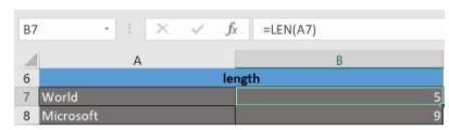
Fig: Len function in Excel

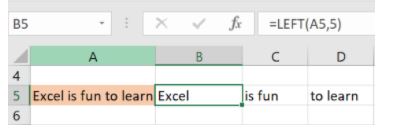
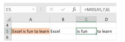
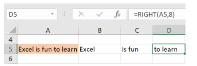
5. LIFT ,RIGHT,MID

The LEFT() function gives the number of characters from the start of a text string. Meanwhile, the MID() function returns the characters from the middle of a text string, given a starting position and length. Finally, the right() function returns the number of characters from the end of a text string.

Let’s understand these functions with a few examples.

In the example below, we use the function left to obtain the leftmost word on the sentence in cell A5.

Shown below is an example using the mid function.

Here, we have an example of the right function.

6.VLOOKUP

Next up in this article is the VLOOKUP() function. This stands for the vertical lookup that is responsible for looking for a particular value in the leftmost column of a table. It then returns a value in the same row from a column you specify.

Below are the arguments for the VLOOKUP function:

lookup_value – This is the value that you have to look for in the first column of a table.

table – This indicates the table from which the value is retrieved.

col_index – The column in the table from the value is to be retrieved.

range_lookup – [optional] TRUE = approximate match (default). FALSE = exact match.

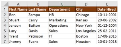
We will use the below table to learn how the VLOOKUP function works.

If you wanted to find the department to which Stuart belongs, you could use the VLOOKUP function as shown below:

excal